How to Make a Synthwave Scene in Blender with Geometry Nodes

阅读本文的中文版本：如何在Blender中使用几何节点制作Synthwave场景

Introduction

Hello, this is Mozi1924! Today, we’ll learn how to create a retro-styled Synthwave scene using Blender’s Geometry Nodes. Transitioning from video to a illustrated tutorial, I hope to bring you a different reading experience. Don’t forget to bookmark my website, mozi1924.com!

In this tutorial, we’ll build this dynamic Synthwave world together:

What are Geometry Nodes?

Geometry Nodes is a powerful tool built into Blender that allows you to generate and modify geometry using a node graph. You can combine various nodes like building blocks, using mathematical logic to create infinitely complex models—and everything is procedural, making later adjustments easy.

What Will You Learn?

This tutorial will guide you through completing a full Synthwave scene, covering these core concepts:

• Creating a base grid with the Grid node
• Controlling grid shape with the Set Position node
• Generating rolling hills using Noise Texture
• Creating a straight highway with Map Range
• Passing data to materials via Store Named Attribute
• Understanding basic math and vector operations

In the material section, we’ll also cover:

• Creating glowing grid effects with Wave Texture
• Controlling color and masks with Color Ramp
• Mixing transparent materials with Mix Shader

Ready? Let’s dive in!

Building the Ground

1. Creating the Base Grid

Add a new plane to the scene (Shift+A → Mesh → Plane). Select it, then open the Geometry Node Editor and click New to create a new node tree.

By default, you’ll see Group Input and Group Output nodes. Let’s delete the Group Input node first. Then, add a Grid node and connect it to the Group Output.

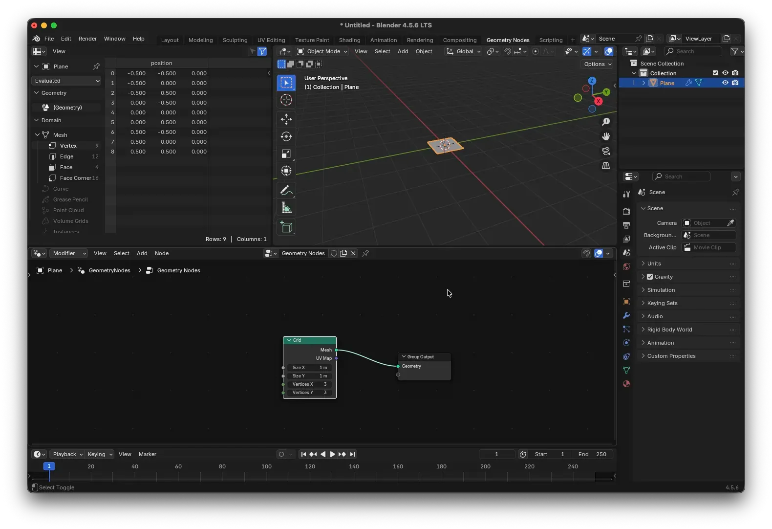
In the Grid node, set both Size X/Y to 200 and Vertices X/Y to 200 to get a sufficiently large grid ground.

2. Sculpting the Terrain

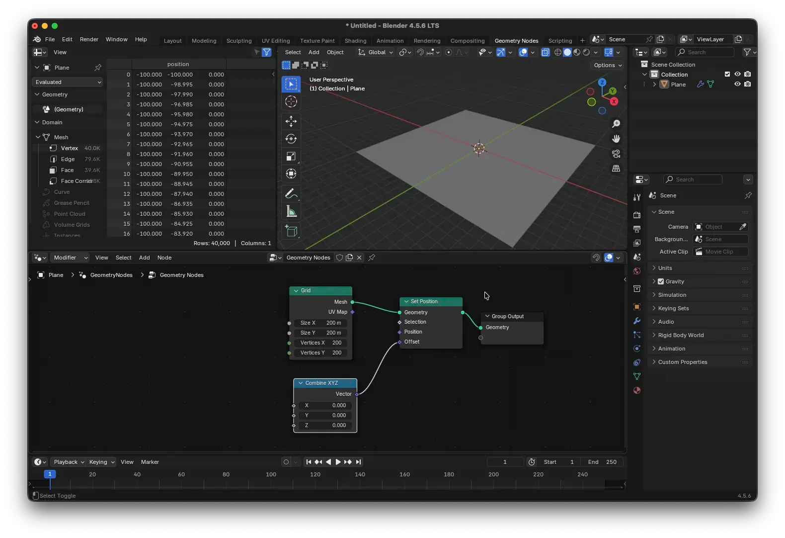
Next, add a Set Position node and place it between the Grid and Group Output. This node allows us to change the position of each vertex.

To control the height (Z-axis), we need a Combine XYZ node. Connect its output to the Offset input of the Set Position node.

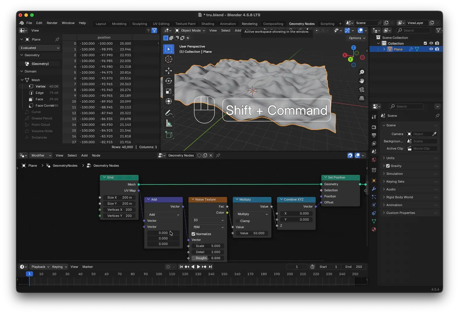
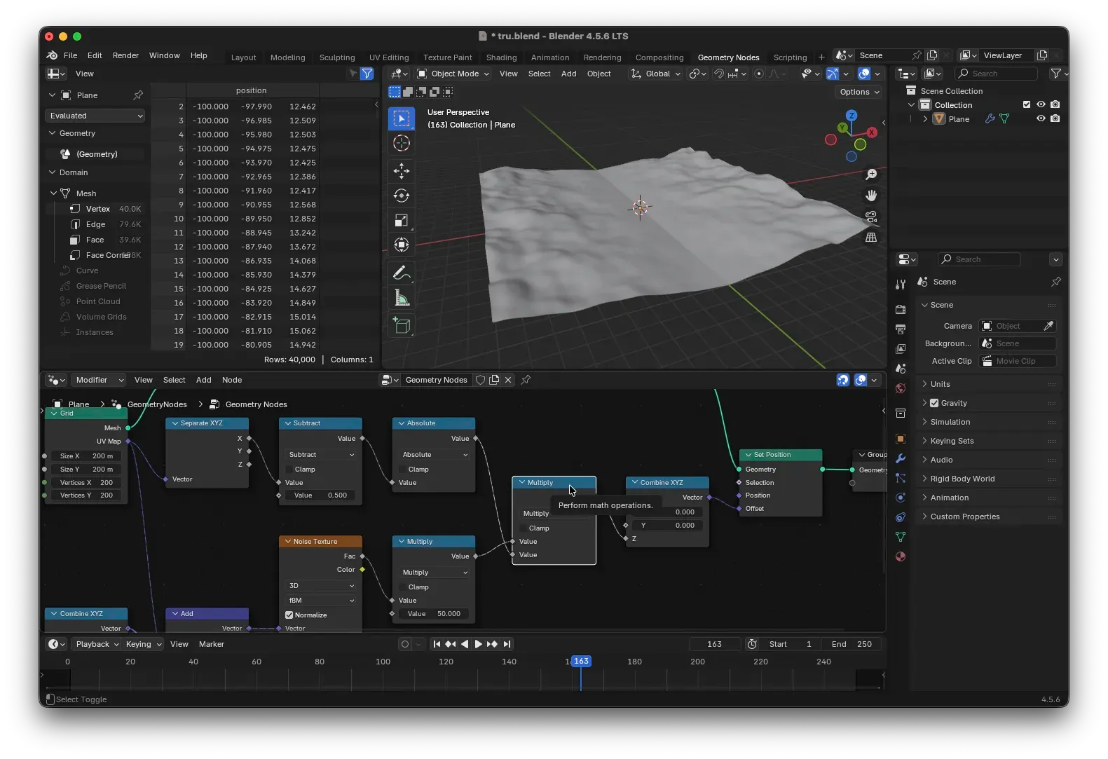
Now, add a Noise Texture node. Connect its Fac output to the Z input of the Combine XYZ node. You’ll notice the ground becomes bumpy with noise—but it doesn’t look like hills yet because the noise lacks positional information.

Connect the UV Map output from the Grid node to the Vector input of the Noise Texture. The noise immediately smooths out, forming natural hill contours.

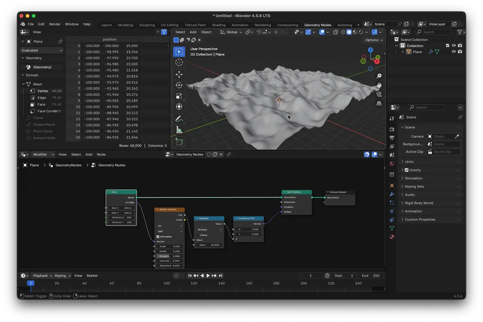
Now, use a Math (Multiply) node to amplify the noise intensity. For example, multiplying by 50 makes the hills prominently visible. You can adjust the noise parameters and the multiplication factor to your liking.

3. Animating the Ground Movement

To create a sense of the ground “moving forward,” we need to make the UV coordinates change over time. Insert a Vector Math node between the Grid and the Noise Texture, setting its operation to Add.

Next, add a Scene Time node. Use a Combine XYZ node to apply its effect only on the Y-axis: connect the Seconds output of Scene Time to the Y input of this new Combine XYZ. Then, connect this Combine XYZ to the second input of the Vector Math node.

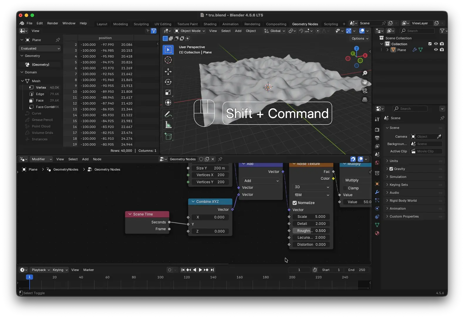
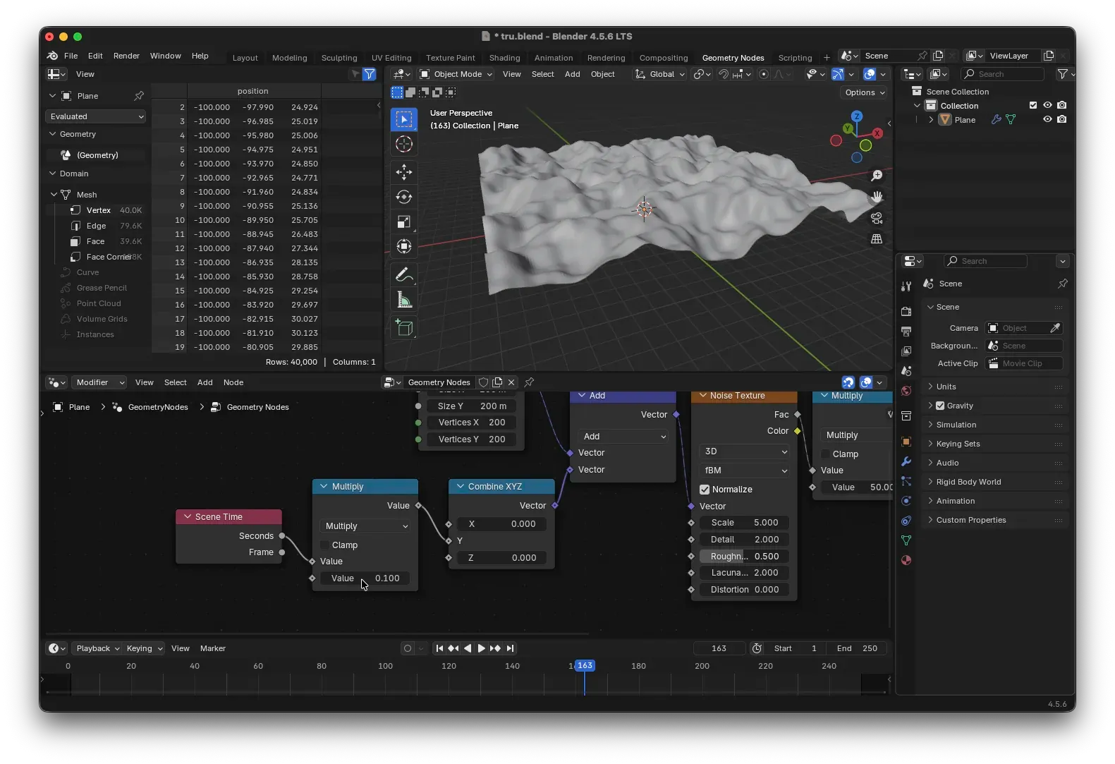
Play the animation (Spacebar). The ground will now move in the positive Y direction. If it’s too fast, insert a Math (Multiply) node in between to multiply the time by a smaller coefficient (e.g., 0.1) to slow it down.

Now that the ground has undulations and motion, let’s carve out a straight highway for it.

Building the Highway

The highway is essentially a depressed strip symmetrical along the X-axis. We’ll generate this mask by separating the axes and applying mathematical operations.

Add a Separate XYZ node, feed the Grid’s UV Map into it, and extract the X-axis. Then:

• First, use a Math (Subtract) node to subtract a value (e.g., 0, to keep the center symmetrical).
• Then, use a Math (Absolute) node to take the absolute value, making the values on both sides of the X-axis symmetrical.

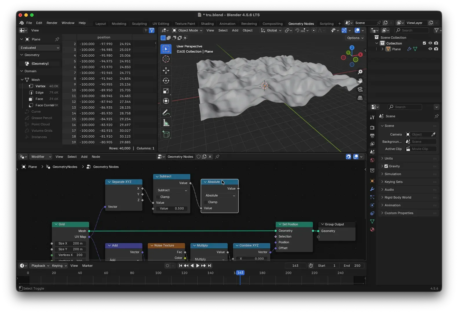
Use this symmetrical value as a coefficient for the height influence: Insert another Math (Multiply) node just before the values enter the Combine XYZ node (after the noise multiplication), and multiply the noise strength by this symmetrical value.

You’ll now see a thin depressed line appear in the center of the ground—the prototype of the highway. However, the line is too thin. We need a Map Range node to adjust its width and falloff.

Connect the Map Range node after the Absolute node. Adjust From Min / Max to control the range of the depression, and To Min / Max to control the intensity of the depression (usually kept at 0–1). For a smoother transition, change the interpolation type to Smooth Step.

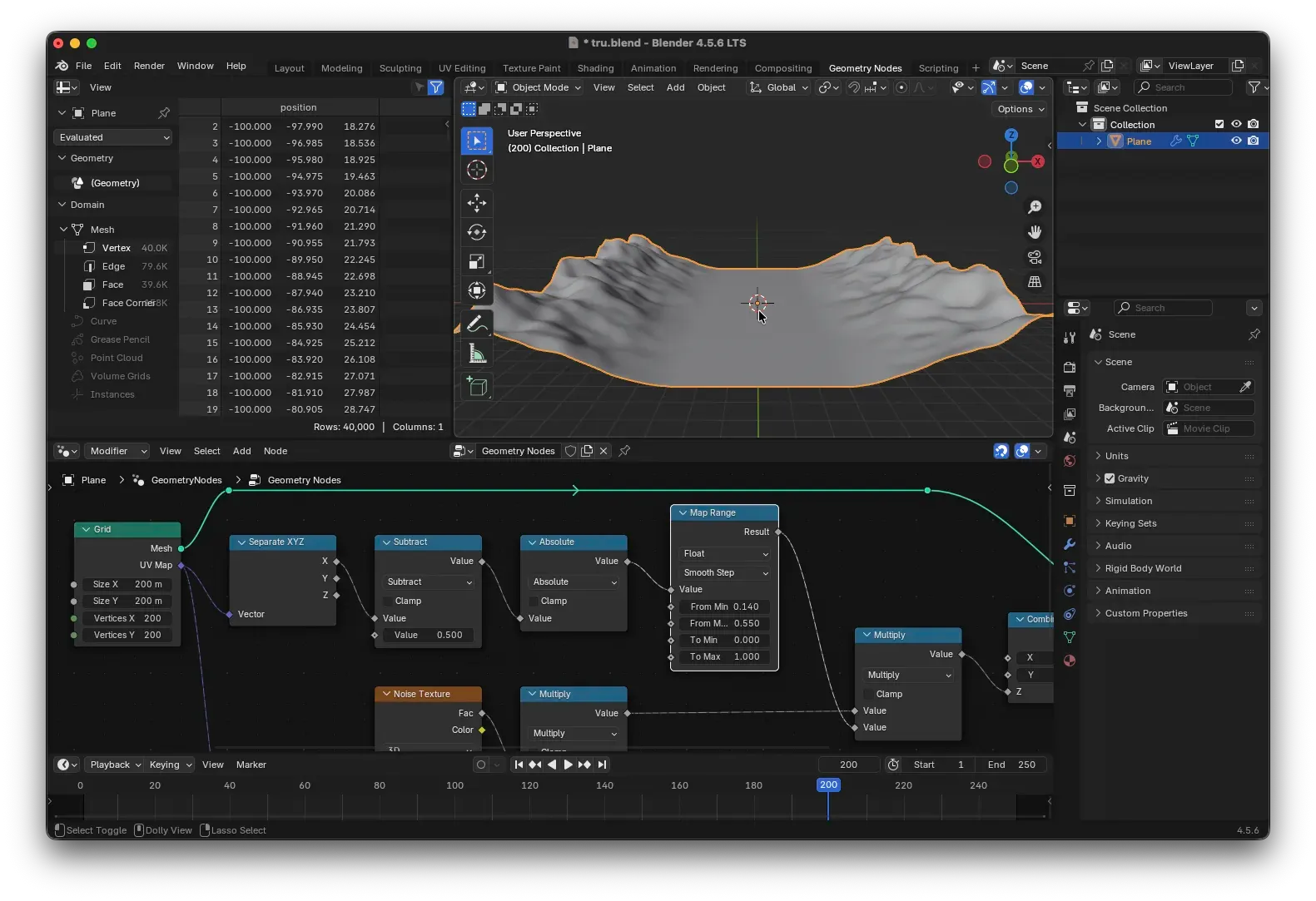
Now, the highway’s depression blends naturally with the hills on either side, and the effect looks quite good.

Passing Data to Materials: Store Named Attribute

To allow the material to also read the moving coordinates of the ground (so the glowing grid moves along with it), we need to “store” the coordinate data within the geometry. This is done using the Store Named Attribute node.

Place it within the geometry data flow (for example, after the Set Position node). Set the data type to Vector and the attribute name to v_pos (or any name you prefer). Connect the coordinate output from our earlier Vector Math node to its Value input.

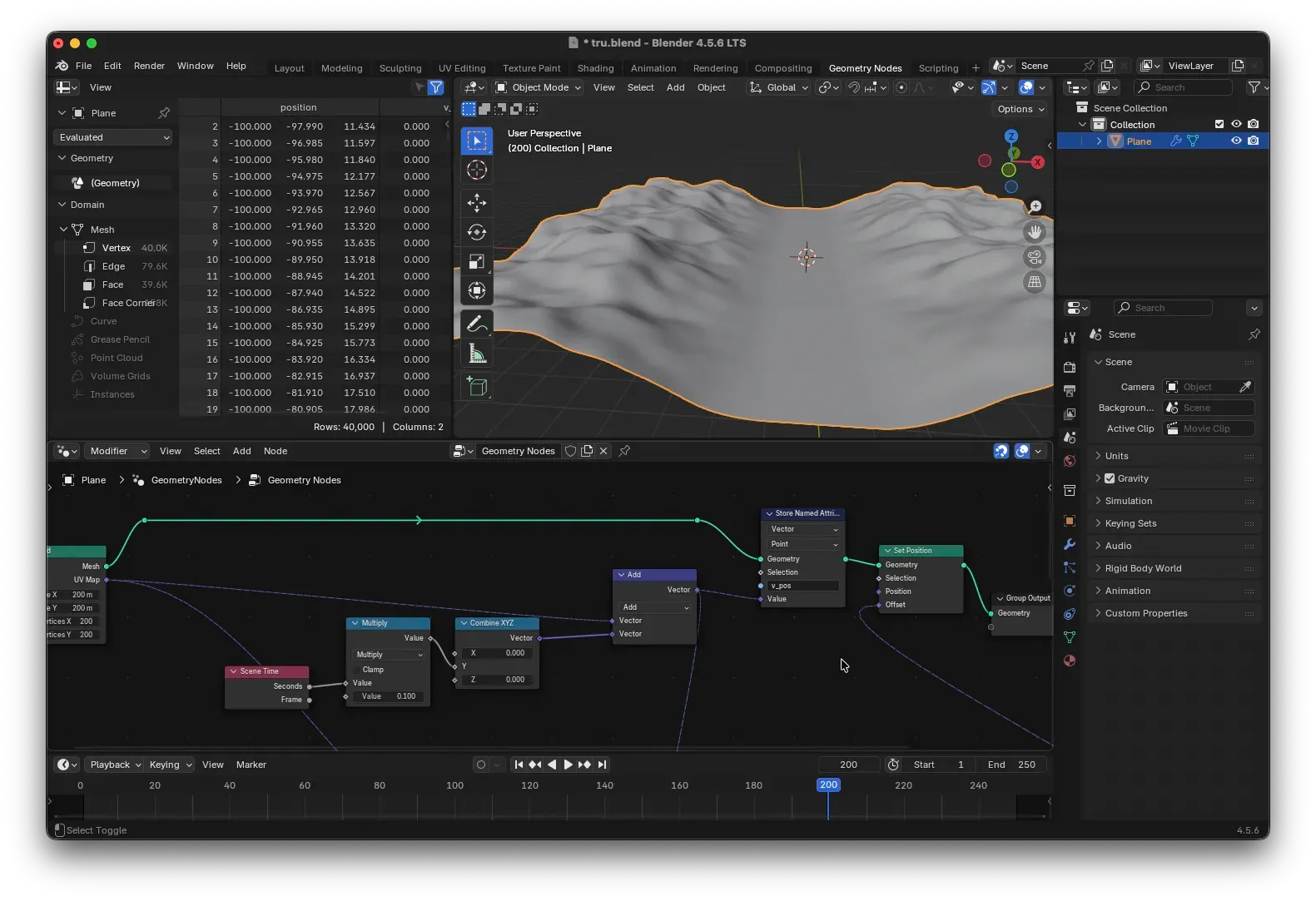
This saves the final position of each vertex into the attribute v_pos, which can be accessed later by shader nodes.

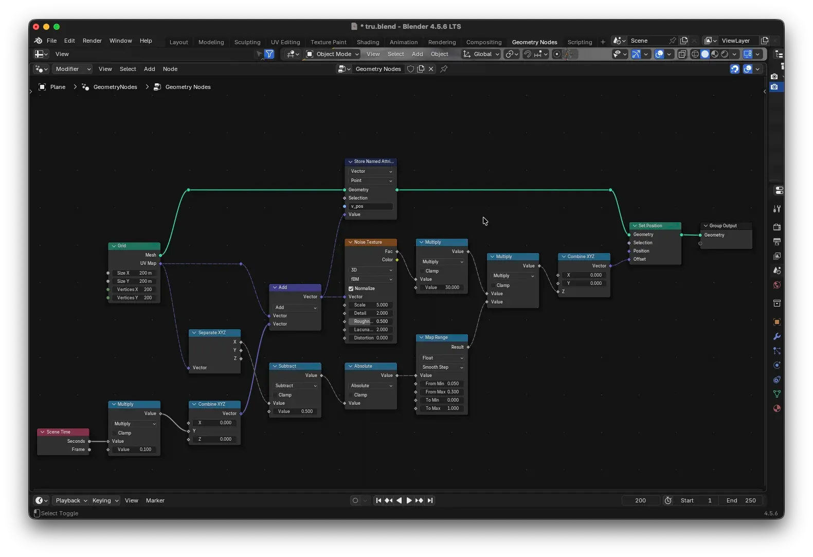
The overall node tree should look something like this:

Don’t forget to add a Set Material node at the end of your Geometry Node tree, pointing to the material we’re about to create. Otherwise, the material won’t be applied.

Ground Material: The Glowing Grid

Switch to the Shader Editor and create a new material. Go back to the Geometry Nodes and assign this material to the ground using the Set Material node.

Now, let’s build the material. Our goal is a glowing grid that conforms perfectly to the terrain’s起伏.

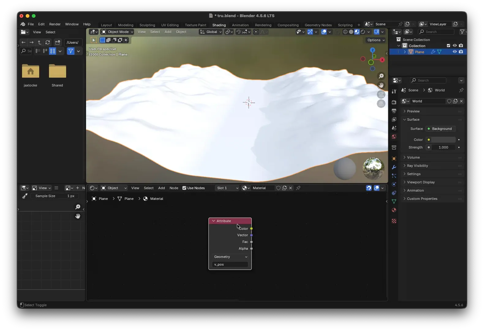
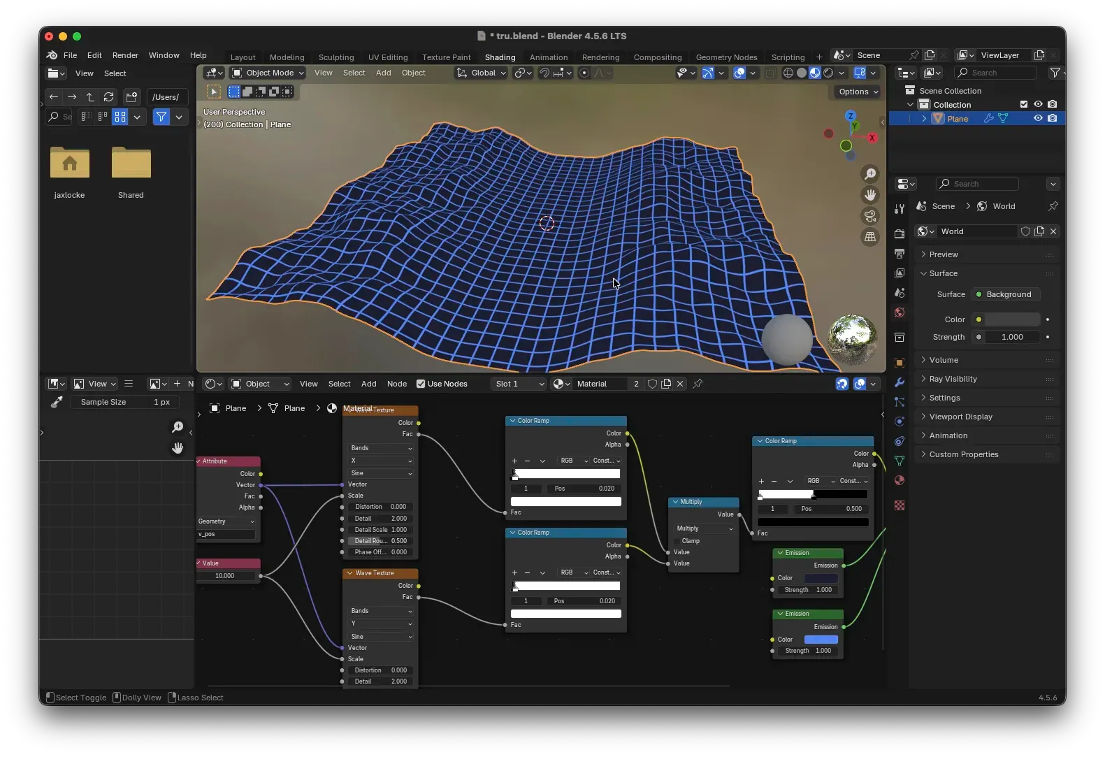
1. Add an Attribute node. Set the Type to Geometry and the Name to v_pos (the name we defined earlier). This gives us the final world coordinates of each vertex (after displacement and movement).
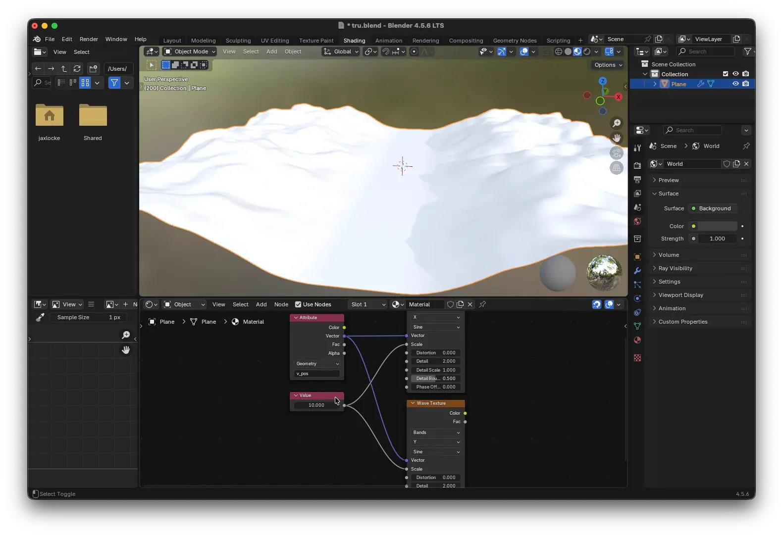
2. Use two Wave Texture nodes to generate stripes in the X and Y directions:
   • First: Bands Direction = X, Wave Profile = Sine
   • Second: Bands Direction = Y, Wave Profile = Sine
   • Use a Value node to control their Scale (e.g., 10), adjusting the grid density.

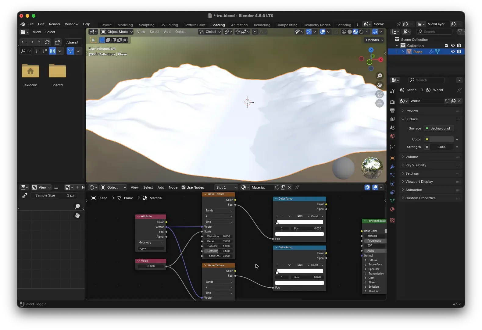
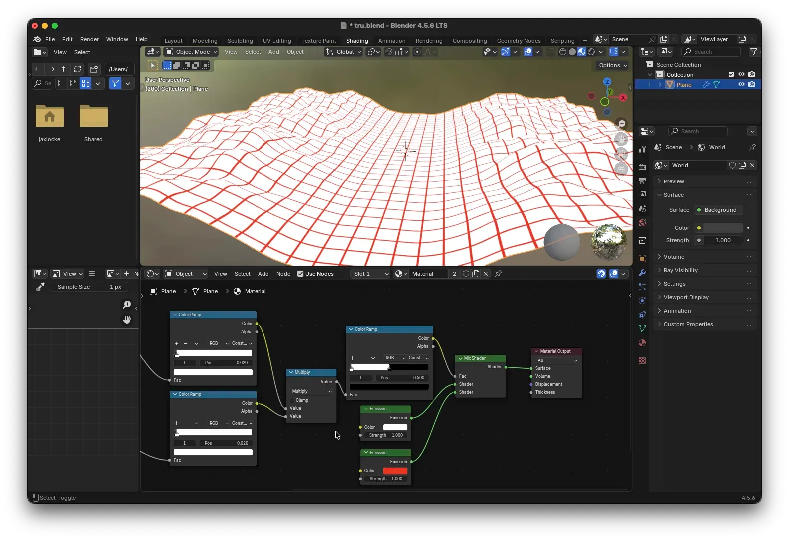
3. Connect each Wave Texture to a Color Ramp. Sharpen the gradient into distinct black and white stripes:
   • Set the first color to pure black (position 0), the second color to pure white (position 0.02). Set the interpolation to Constant.
   • This retains only a small segment around the wave peaks as white, turning the rest black, creating thin lines.

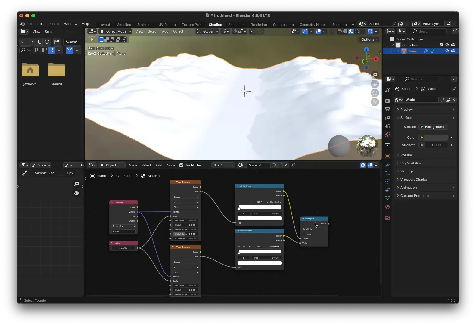
4. Multiply the outputs of the two Color Ramps using a Math (Multiply) node. This gives us the intersecting grid pattern (the white parts are the grid lines).

5. Add another Color Ramp to convert the multiplied result into a hard mask: set the first color to pure white, the second to pure black. Use Constant interpolation, and set the position of the second color to 0.5. This makes areas brighter than 0.5 white (grid lines) and everything else black.

6. Create two Emission nodes. Set their colors to your preference (e.g., purple and magenta). Mix them using a Mix Shader, with the factor (Fac) driven by the mask from the previous step.

Finally, you’ll see the glowing grid perfectly贴合 the ground’s起伏 and moving along with it. Adjust the earlier Value node to change the grid density, and feel free to experiment with the colors of the two Emission shaders.

Creating the Retro Sun

The iconic visual element of Synthwave—the louvered sunset—can be achieved with a simple sphere and a procedural material.

1. Basic Setup

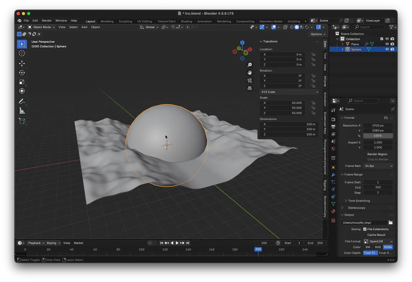
Add a UV sphere to the scene (Shift+A → Mesh → UV Sphere). Right-click and choose Shade Smooth. Set the sphere’s scale to (50, 0.01, 50)—squashing it on the Y-axis to form a flat disc, making the stripe effect easier to observe. Position it appropriately in the background of the scene.

2. Material Concept

This material can be broken down into two parts: a vertical color gradient and horizontal transparent stripes.

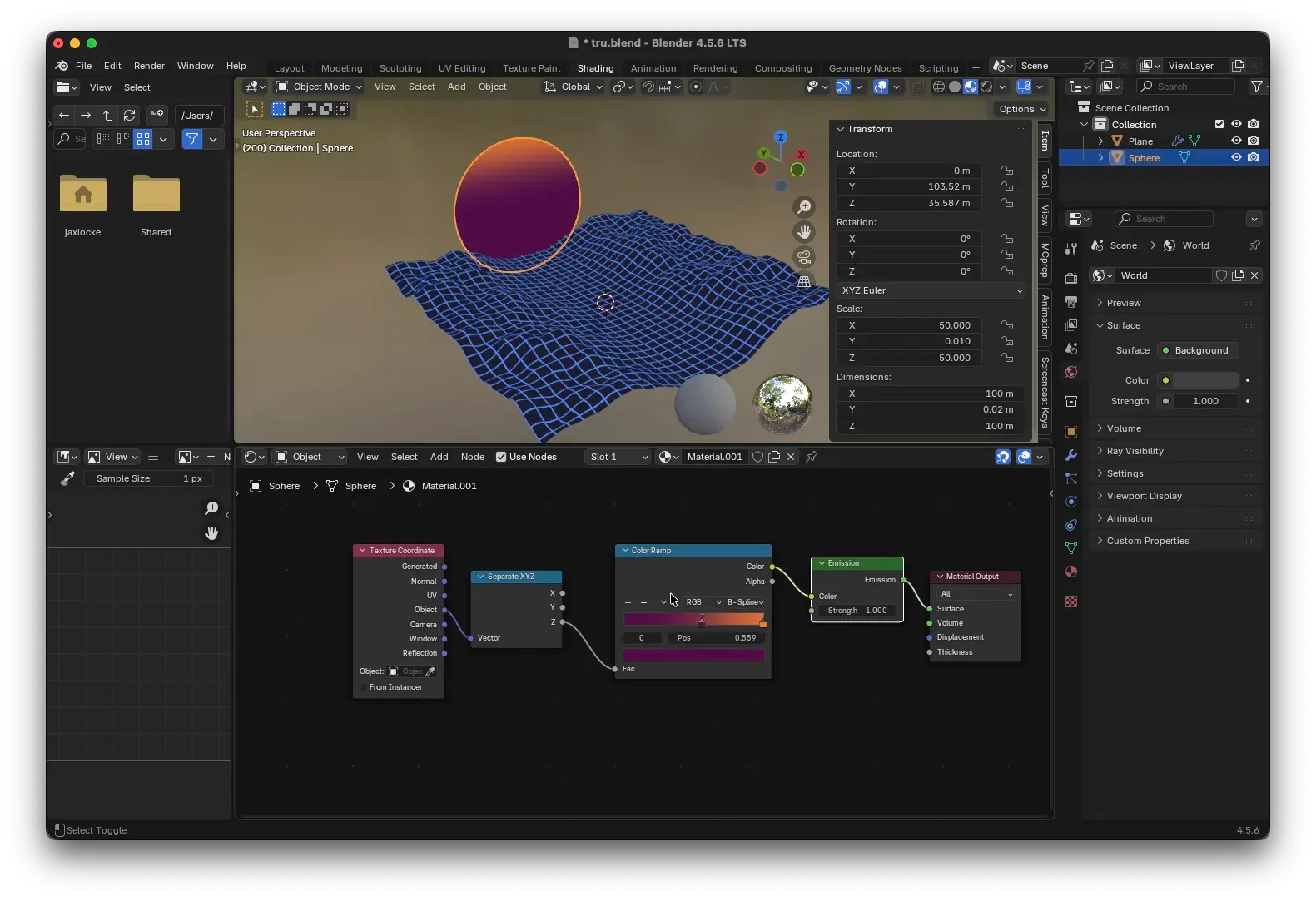
3. Getting Coordinates and Separating Z

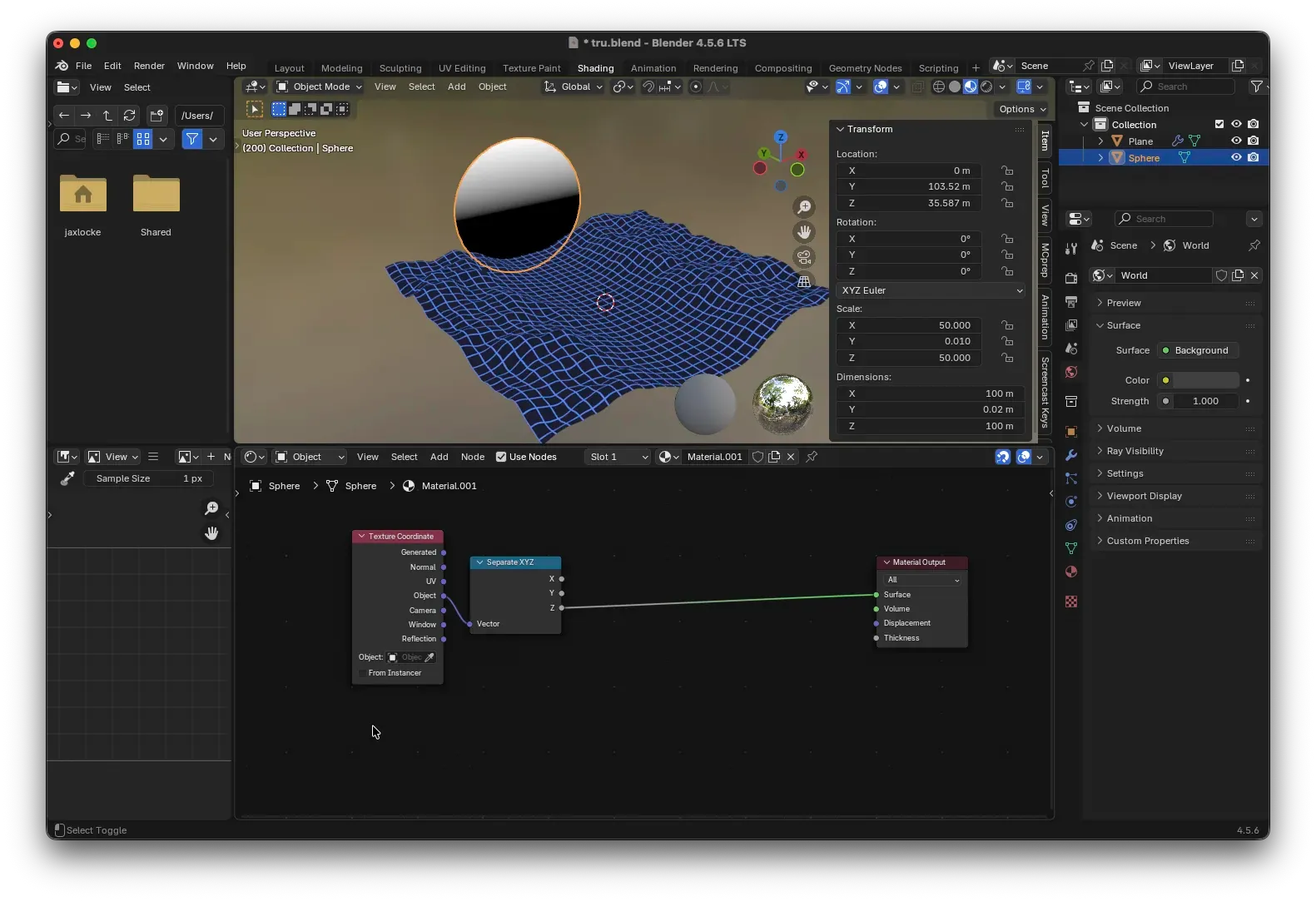
Create a new material. Add a Texture Coordinate node and use its Object output. Since we want the gradient based on the object’s own Z-axis (up-down direction), using Object coordinates ensures that the Z-axis always points along the object’s local up direction, regardless of rotation.

Add a Separate XYZ node and extract the Z-axis. At this point, the black-and-white gradient maps from bottom (black) to top (white).

4. Creating the Color Gradient

Feed the Z-axis into a Color Ramp. Set two color stops:

• Left side (bottom): Dark purple or black
• Right side (top): Bright orange or yellow

Connect the Color Ramp output to an Emission node. Increase the strength slightly (e.g., 1.0~2.0) to make the sun glow.

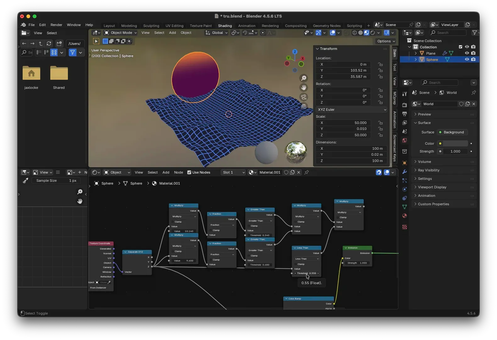
5. Math Combination: Making the Stripes

We need to turn the continuous Z-axis into间断的 stripes. This uses a classic series of math operations: Multiply → Fraction → Compare.

• Multiply: Controls the stripe density. In the example, two branches are used, multiplying by slightly different values like 10.14 and 9.60. This叠加 two slightly different frequencies, preventing the stripes from looking too rigid and creating more interesting detail.
• Fraction: Takes the fractional part of the value, turning the continuous line into a repeating sawtooth wave.
• Greater Than: Sets a threshold (e.g., 0.5). It binarizes the sawtooth wave: outputs 1 (white) where the value is greater than the threshold, otherwise 0 (black). Adjusting the threshold controls the stripe thickness.

Multiply the results of the two branches using a Multiply node to get the final stripe mask (white areas will be transparent, black areas will glow). Finally, you might use a Less Than node to invert the mask if needed, depending on how you want it to drive the Mix Shader factor (0=glow, 1=transparent).

6. Mixing Transparency

Add a Mix Shader node:

• Shader 1 input: Connect our finished Emission node.
• Shader 2 input: Connect a Transparent BSDF node.
• Fac input: Connect the output from the mathematical operations (the final mask).

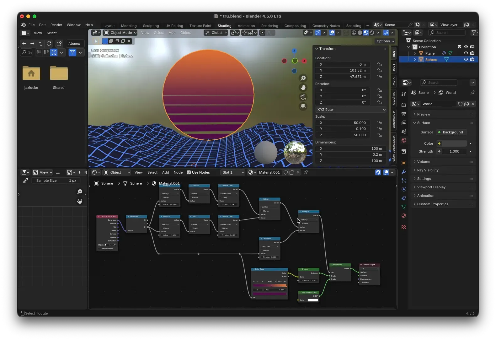
Now, where the factor is 0, the glowing sun is visible. Where the factor is 1, transparency is shown, effectively “cutting” stripes out of the sun and creating the classic louvered effect.

Feel free to adjust the colors, stripe density, and thickness to create your own unique retro sunset.

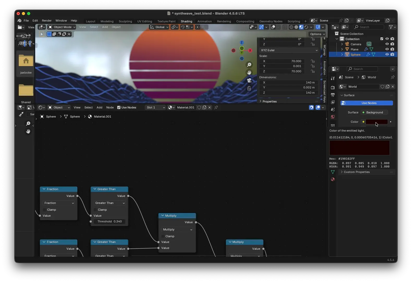
Sky

In the Properties panel on the side, click on the World properties. Set the background color to a dark purple or any other color you like.

Conclusion

With this, we’ve completed the modeling and material creation for the entire Synthwave scene. From the procedural terrain in Geometry Nodes to the dynamic grid and striped sun in the Shader Editor, each step blends mathematics and aesthetics. I hope this tutorial helps you better master Blender’s Geometry Nodes and Shader Nodes, and inspires you to create even more interesting projects!

If you enjoyed this tutorial, don’t forget to bookmark my website, mozi1924.com. More exciting content is on the way. See you next time!